Create grids and calculate statistics
Usage
lsm_grid_statistic(
  input,
  output = NULL,
  landscape_metric,
  landscape_metric_has_null = FALSE,
  size,
  hexagon = FALSE,
  column_prefix,
  method = "average",
  percentile = NULL
)
Arguments
- input
[character=""]- output
[character=""]
Map name output inside GRASS Data Base.- landscape_metric
[character=""]- landscape_metric_has_null
[character=""]- size
[character=""]- hexagon
[character=""]- column_prefix
[character=""]- method
[character=""]
Univariate statistics: number, null_cells, minimum ,maximum, range, average, stddev, variance, coeff_var, sum, first_quartile ,median, third_quartile, percentile- percentile
[character=""]
Examples
library(lsmetrics)
library(terra)
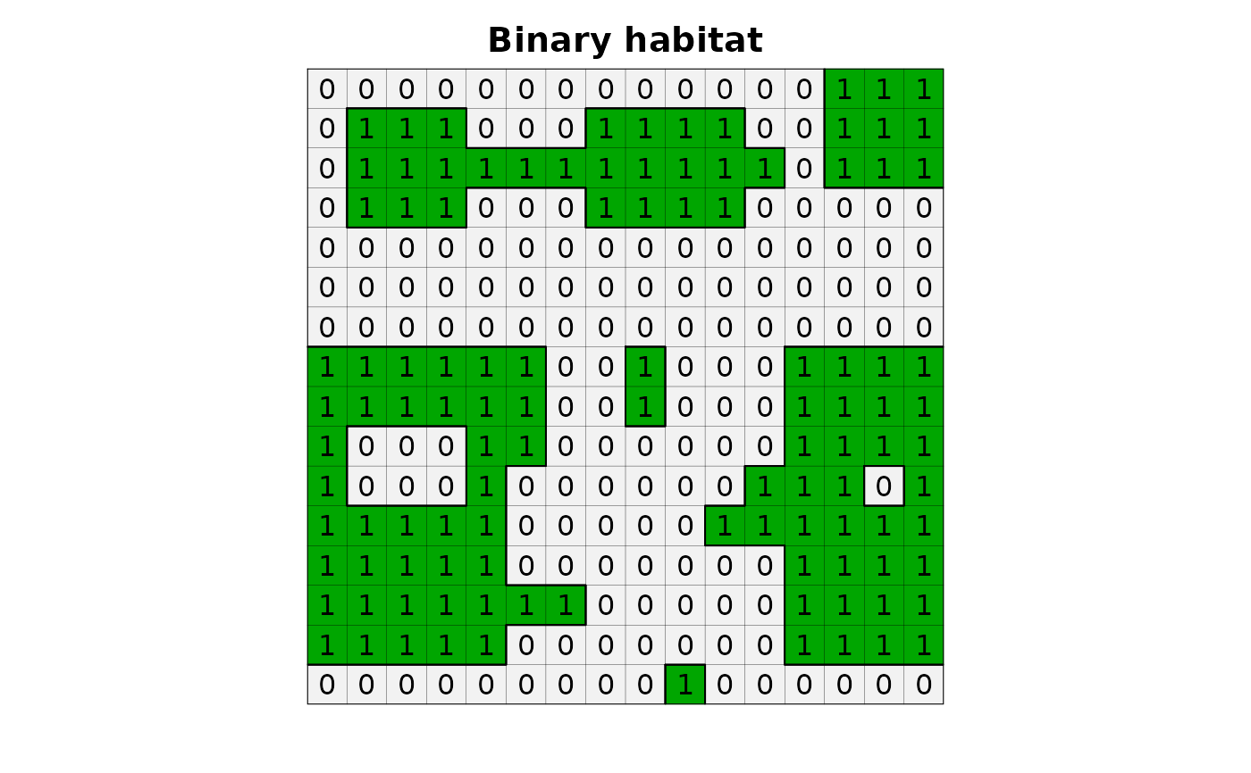
# read habitat data
f <- system.file("raster/toy_landscape_habitat.tif", package = "lsmetrics")
r <- terra::rast(f)
# plot
plot(r, legend = FALSE, axes = FALSE, main = "Binary habitat")
plot(as.polygons(r, dissolve = FALSE), lwd = .1, add = TRUE)
plot(as.polygons(r), add = TRUE)
text(r)
 # find grass
path_grass <- system("grass --config path", inter = TRUE) # windows users need to find the grass gis path installation, e.g. "C:/Program Files/GRASS GIS 8.3"
# create grassdb
rgrass::initGRASS(gisBase = path_grass,
SG = r,
gisDbase = "grassdb",
location = "newLocation",
mapset = "PERMANENT",
override = TRUE)
#> gisdbase grassdb
#> location newLocation
#> mapset PERMANENT
#> rows 16
#> columns 16
#> north 7525600
#> south 7524000
#> west 234000
#> east 235600
#> nsres 100
#> ewres 100
#> projection:
#> PROJCRS["WGS 84 / UTM zone 23S",
#> BASEGEOGCRS["WGS 84",
#> ENSEMBLE["World Geodetic System 1984 ensemble",
#> MEMBER["World Geodetic System 1984 (Transit)"],
#> MEMBER["World Geodetic System 1984 (G730)"],
#> MEMBER["World Geodetic System 1984 (G873)"],
#> MEMBER["World Geodetic System 1984 (G1150)"],
#> MEMBER["World Geodetic System 1984 (G1674)"],
#> MEMBER["World Geodetic System 1984 (G1762)"],
#> MEMBER["World Geodetic System 1984 (G2139)"],
#> ELLIPSOID["WGS 84",6378137,298.257223563,
#> LENGTHUNIT["metre",1]],
#> ENSEMBLEACCURACY[2.0]],
#> PRIMEM["Greenwich",0,
#> ANGLEUNIT["degree",0.0174532925199433]],
#> ID["EPSG",4326]],
#> CONVERSION["UTM zone 23S",
#> METHOD["Transverse Mercator",
#> ID["EPSG",9807]],
#> PARAMETER["Latitude of natural origin",0,
#> ANGLEUNIT["degree",0.0174532925199433],
#> ID["EPSG",8801]],
#> PARAMETER["Longitude of natural origin",-45,
#> ANGLEUNIT["degree",0.0174532925199433],
#> ID["EPSG",8802]],
#> PARAMETER["Scale factor at natural origin",0.9996,
#> SCALEUNIT["unity",1],
#> ID["EPSG",8805]],
#> PARAMETER["False easting",500000,
#> LENGTHUNIT["metre",1],
#> ID["EPSG",8806]],
#> PARAMETER["False northing",10000000,
#> LENGTHUNIT["metre",1],
#> ID["EPSG",8807]]],
#> CS[Cartesian,2],
#> AXIS["(E)",east,
#> ORDER[1],
#> LENGTHUNIT["metre",1]],
#> AXIS["(N)",north,
#> ORDER[2],
#> LENGTHUNIT["metre",1]],
#> USAGE[
#> SCOPE["Navigation and medium accuracy spatial referencing."],
#> AREA["Between 48°W and 42°W, southern hemisphere between 80°S and equator, onshore and offshore. Brazil."],
#> BBOX[-80,-48,0,-42]],
#> ID["EPSG",32723]]
# import raster from r to grass
rgrass::write_RAST(x = r, flags = c("o", "overwrite", "quiet"), vname = "r", verbose = FALSE)
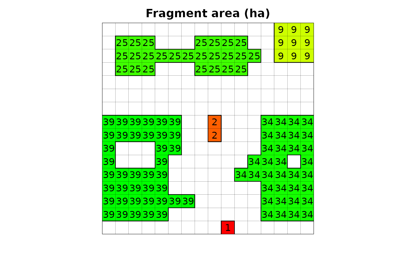
# area
lsmetrics::lsm_fragment_area(input = "r")
#> Converting zero as null
#> Identifying the fragmentes
#> Counting the cell number of fragmentes
#> First pass
#> 0% 6% 12% 18% 25% 31% 37% 43% 50% 56% 62% 68% 75% 81% 87% 93% 100%
#> Writing output map
#> 0% 6% 12% 18% 25% 31% 37% 43% 50% 56% 62% 68% 75% 81% 87% 93% 100%
#> Calculating the area of fragmentes
# files
# rgrass::execGRASS(cmd = "g.list", type = "raster")
# import r
r_fragment_area_ha <- rgrass::read_RAST("r_fragment_area_ha", flags = "quiet")
# plot
plot(r_fragment_area_ha, legend = FALSE, axes = FALSE, main = "Fragment area (ha)")
plot(as.polygons(r, dissolve = FALSE), lwd = .1, add = TRUE)
plot(as.polygons(r), add = TRUE)
text(r_fragment_area_ha)
# find grass
path_grass <- system("grass --config path", inter = TRUE) # windows users need to find the grass gis path installation, e.g. "C:/Program Files/GRASS GIS 8.3"
# create grassdb
rgrass::initGRASS(gisBase = path_grass,
SG = r,
gisDbase = "grassdb",
location = "newLocation",
mapset = "PERMANENT",
override = TRUE)
#> gisdbase grassdb
#> location newLocation
#> mapset PERMANENT
#> rows 16
#> columns 16
#> north 7525600
#> south 7524000
#> west 234000
#> east 235600
#> nsres 100
#> ewres 100
#> projection:
#> PROJCRS["WGS 84 / UTM zone 23S",
#> BASEGEOGCRS["WGS 84",
#> ENSEMBLE["World Geodetic System 1984 ensemble",
#> MEMBER["World Geodetic System 1984 (Transit)"],
#> MEMBER["World Geodetic System 1984 (G730)"],
#> MEMBER["World Geodetic System 1984 (G873)"],
#> MEMBER["World Geodetic System 1984 (G1150)"],
#> MEMBER["World Geodetic System 1984 (G1674)"],
#> MEMBER["World Geodetic System 1984 (G1762)"],
#> MEMBER["World Geodetic System 1984 (G2139)"],
#> ELLIPSOID["WGS 84",6378137,298.257223563,
#> LENGTHUNIT["metre",1]],
#> ENSEMBLEACCURACY[2.0]],
#> PRIMEM["Greenwich",0,
#> ANGLEUNIT["degree",0.0174532925199433]],
#> ID["EPSG",4326]],
#> CONVERSION["UTM zone 23S",
#> METHOD["Transverse Mercator",
#> ID["EPSG",9807]],
#> PARAMETER["Latitude of natural origin",0,
#> ANGLEUNIT["degree",0.0174532925199433],
#> ID["EPSG",8801]],
#> PARAMETER["Longitude of natural origin",-45,
#> ANGLEUNIT["degree",0.0174532925199433],
#> ID["EPSG",8802]],
#> PARAMETER["Scale factor at natural origin",0.9996,
#> SCALEUNIT["unity",1],
#> ID["EPSG",8805]],
#> PARAMETER["False easting",500000,
#> LENGTHUNIT["metre",1],
#> ID["EPSG",8806]],
#> PARAMETER["False northing",10000000,
#> LENGTHUNIT["metre",1],
#> ID["EPSG",8807]]],
#> CS[Cartesian,2],
#> AXIS["(E)",east,
#> ORDER[1],
#> LENGTHUNIT["metre",1]],
#> AXIS["(N)",north,
#> ORDER[2],
#> LENGTHUNIT["metre",1]],
#> USAGE[
#> SCOPE["Navigation and medium accuracy spatial referencing."],
#> AREA["Between 48°W and 42°W, southern hemisphere between 80°S and equator, onshore and offshore. Brazil."],
#> BBOX[-80,-48,0,-42]],
#> ID["EPSG",32723]]
# import raster from r to grass
rgrass::write_RAST(x = r, flags = c("o", "overwrite", "quiet"), vname = "r", verbose = FALSE)
# area
lsmetrics::lsm_fragment_area(input = "r")
#> Converting zero as null
#> Identifying the fragmentes
#> Counting the cell number of fragmentes
#> First pass
#> 0% 6% 12% 18% 25% 31% 37% 43% 50% 56% 62% 68% 75% 81% 87% 93% 100%
#> Writing output map
#> 0% 6% 12% 18% 25% 31% 37% 43% 50% 56% 62% 68% 75% 81% 87% 93% 100%
#> Calculating the area of fragmentes
# files
# rgrass::execGRASS(cmd = "g.list", type = "raster")
# import r
r_fragment_area_ha <- rgrass::read_RAST("r_fragment_area_ha", flags = "quiet")
# plot
plot(r_fragment_area_ha, legend = FALSE, axes = FALSE, main = "Fragment area (ha)")
plot(as.polygons(r, dissolve = FALSE), lwd = .1, add = TRUE)
plot(as.polygons(r), add = TRUE)
text(r_fragment_area_ha)
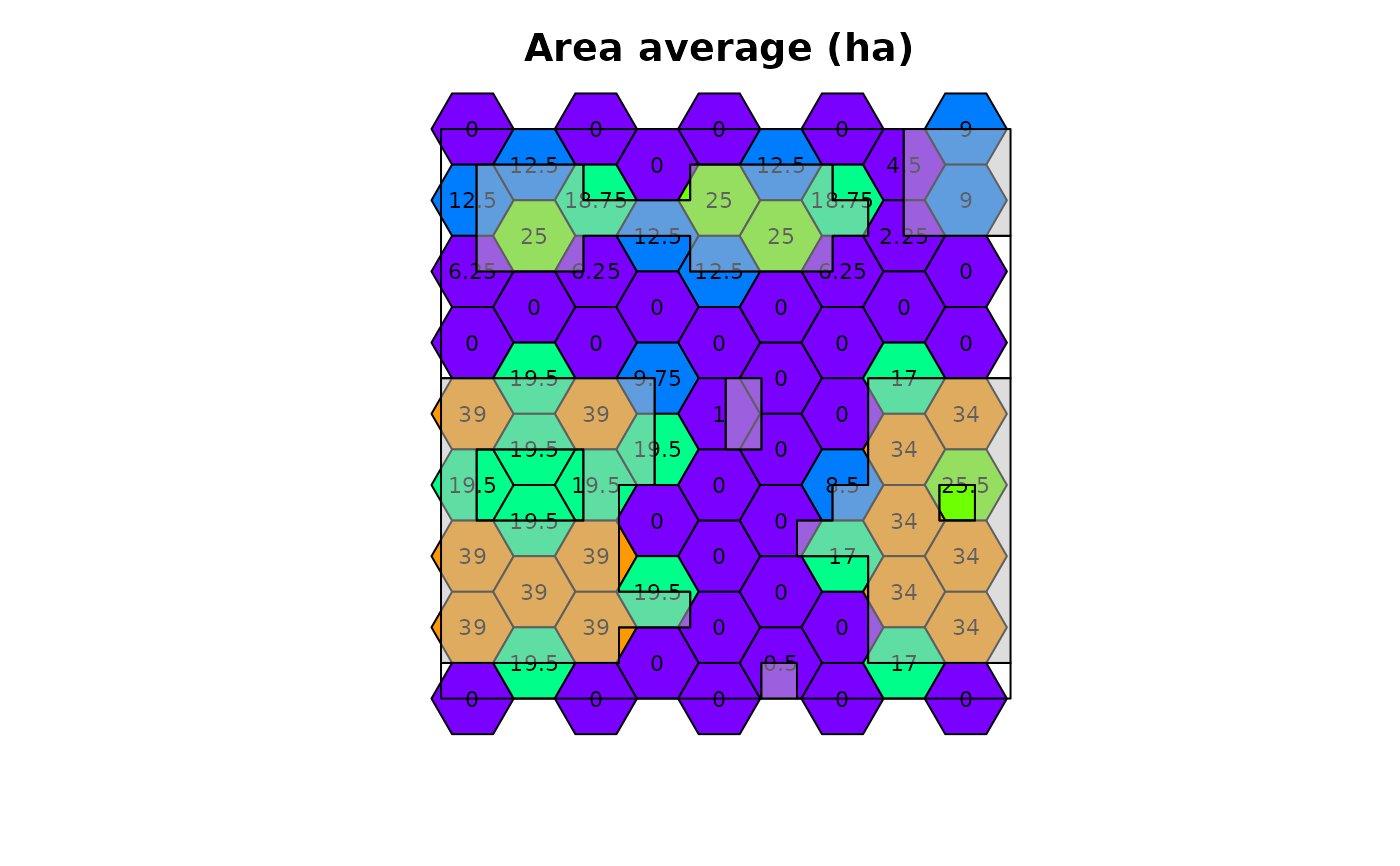
 # grid
lsmetrics::lsm_grid_statistic(input = "r",
landscape_metric = "r_fragment_area_ha",
landscape_metric_has_null = TRUE,
size = 200,
hexagon = TRUE,
column_prefix = "area",
method = "average")
#> Using native format
#> Default driver / database set to:
#> driver: sqlite
#> database: $GISDBASE/$LOCATION_NAME/$MAPSET/sqlite/sqlite.db
#> The number of columns has been adjusted from 10 to 11
#> Writing out hexagon grid...
#> 0% 10% 21% 31% 42% 52% 63% 73% 84% 94% 100%
#> Building topology for vector map <r_grid200@PERMANENT>...
#> Registering primitives...
#>
#> 461 primitives registered
#> 817 vertices registered
#> Building areas...
#> 0% 2% 4% 6% 8% 10% 12% 14% 16% 18% 20% 22% 24% 26% 28% 30% 32% 34% 36% 38% 40% 42% 44% 46% 48% 50% 52% 54% 56% 58% 60% 62% 64% 66% 68% 70% 72% 74% 76% 78% 80% 82% 84% 86% 88% 90% 92% 94% 96% 98% 100%
#> 105 areas built
#> One isle built
#> Attaching islands...
#> 0% 100%
#> Attaching centroids...
#> 0% 2% 4% 6% 8% 10% 12% 14% 16% 18% 20% 22% 24% 26% 28% 30% 32% 34% 36% 38% 40% 42% 44% 46% 48% 50% 52% 54% 56% 58% 60% 62% 64% 66% 68% 70% 72% 74% 76% 78% 80% 82% 84% 86% 88% 90% 92% 94% 96% 98% 100%
#> Topology was built
#> Number of nodes: 252
#> Number of primitives: 461
#> Number of points: 0
#> Number of lines: 0
#> Number of boundaries: 356
#> Number of centroids: 105
#> Number of areas: 105
#> Number of isles: 1
# files
# rgrass::execGRASS(cmd = "g.list", type = "vector")
# import r
r_grid <- rgrass::read_VECT("r_grid200", flags = "quiet")
# plot
r_grid <- r_grid[is.na(r_grid$area_average) == FALSE, ]
plot(r_grid, "area_average", legend = FALSE, axes = FALSE, main = "Area average (ha)")
text(r_grid, labels = "area_average", cex = .7)
plot(as.polygons(r), col = c(adjustcolor("white", 0), adjustcolor("gray", .5)), add = TRUE)
# grid
lsmetrics::lsm_grid_statistic(input = "r",
landscape_metric = "r_fragment_area_ha",
landscape_metric_has_null = TRUE,
size = 200,
hexagon = TRUE,
column_prefix = "area",
method = "average")
#> Using native format
#> Default driver / database set to:
#> driver: sqlite
#> database: $GISDBASE/$LOCATION_NAME/$MAPSET/sqlite/sqlite.db
#> The number of columns has been adjusted from 10 to 11
#> Writing out hexagon grid...
#> 0% 10% 21% 31% 42% 52% 63% 73% 84% 94% 100%
#> Building topology for vector map <r_grid200@PERMANENT>...
#> Registering primitives...
#>
#> 461 primitives registered
#> 817 vertices registered
#> Building areas...
#> 0% 2% 4% 6% 8% 10% 12% 14% 16% 18% 20% 22% 24% 26% 28% 30% 32% 34% 36% 38% 40% 42% 44% 46% 48% 50% 52% 54% 56% 58% 60% 62% 64% 66% 68% 70% 72% 74% 76% 78% 80% 82% 84% 86% 88% 90% 92% 94% 96% 98% 100%
#> 105 areas built
#> One isle built
#> Attaching islands...
#> 0% 100%
#> Attaching centroids...
#> 0% 2% 4% 6% 8% 10% 12% 14% 16% 18% 20% 22% 24% 26% 28% 30% 32% 34% 36% 38% 40% 42% 44% 46% 48% 50% 52% 54% 56% 58% 60% 62% 64% 66% 68% 70% 72% 74% 76% 78% 80% 82% 84% 86% 88% 90% 92% 94% 96% 98% 100%
#> Topology was built
#> Number of nodes: 252
#> Number of primitives: 461
#> Number of points: 0
#> Number of lines: 0
#> Number of boundaries: 356
#> Number of centroids: 105
#> Number of areas: 105
#> Number of isles: 1
# files
# rgrass::execGRASS(cmd = "g.list", type = "vector")
# import r
r_grid <- rgrass::read_VECT("r_grid200", flags = "quiet")
# plot
r_grid <- r_grid[is.na(r_grid$area_average) == FALSE, ]
plot(r_grid, "area_average", legend = FALSE, axes = FALSE, main = "Area average (ha)")
text(r_grid, labels = "area_average", cex = .7)
plot(as.polygons(r), col = c(adjustcolor("white", 0), adjustcolor("gray", .5)), add = TRUE)
 # delete grassdb
unlink("grassdb", recursive = TRUE)
# delete grassdb
unlink("grassdb", recursive = TRUE)