Calculate functional connectivity
Source:R/lsm_functional_connectivity.R
lsm_functional_connectivity.RdIdentifies functional fragmentes connected and calculate area in hectare.
Usage
lsm_functional_connectivity(
  input,
  output = NULL,
  zero_as_na = FALSE,
  gap_crossing,
  id = FALSE,
  ncell = FALSE,
  area_integer = FALSE,
  dilation = FALSE,
  dilation_type = "minimum",
  nprocs = 1,
  memory = 300
)
Arguments
- input
[character=""]
Habitat map, following a binary classification (e.g. values 1,0 or 1,NA for habitat,non-habitat).- output
[character=""]
Habitat area map name output GRASS Data Base- zero_as_na
[logical(1)=FALSE]
IfTRUE, the function treats non-habitat cells as null; ifFALSE, the function converts non-habitat zero cells to null cells.- gap_crossing
[numeric]
Integer indicating gap crossing distance.- id
[logical(1)=FALSE]
IfTRUE- ncell
[logical(1)=FALSE]
IfTRUE- area_integer
[logical(1)=FALSE]
IfTRUE- dilation
[logical(1)=FALSE]
IfTRUE- dilation_type
[character=""]
If- nprocs
[numeric()]- memory
[numeric()]
Examples
library(lsmetrics)
library(terra)
# read habitat data
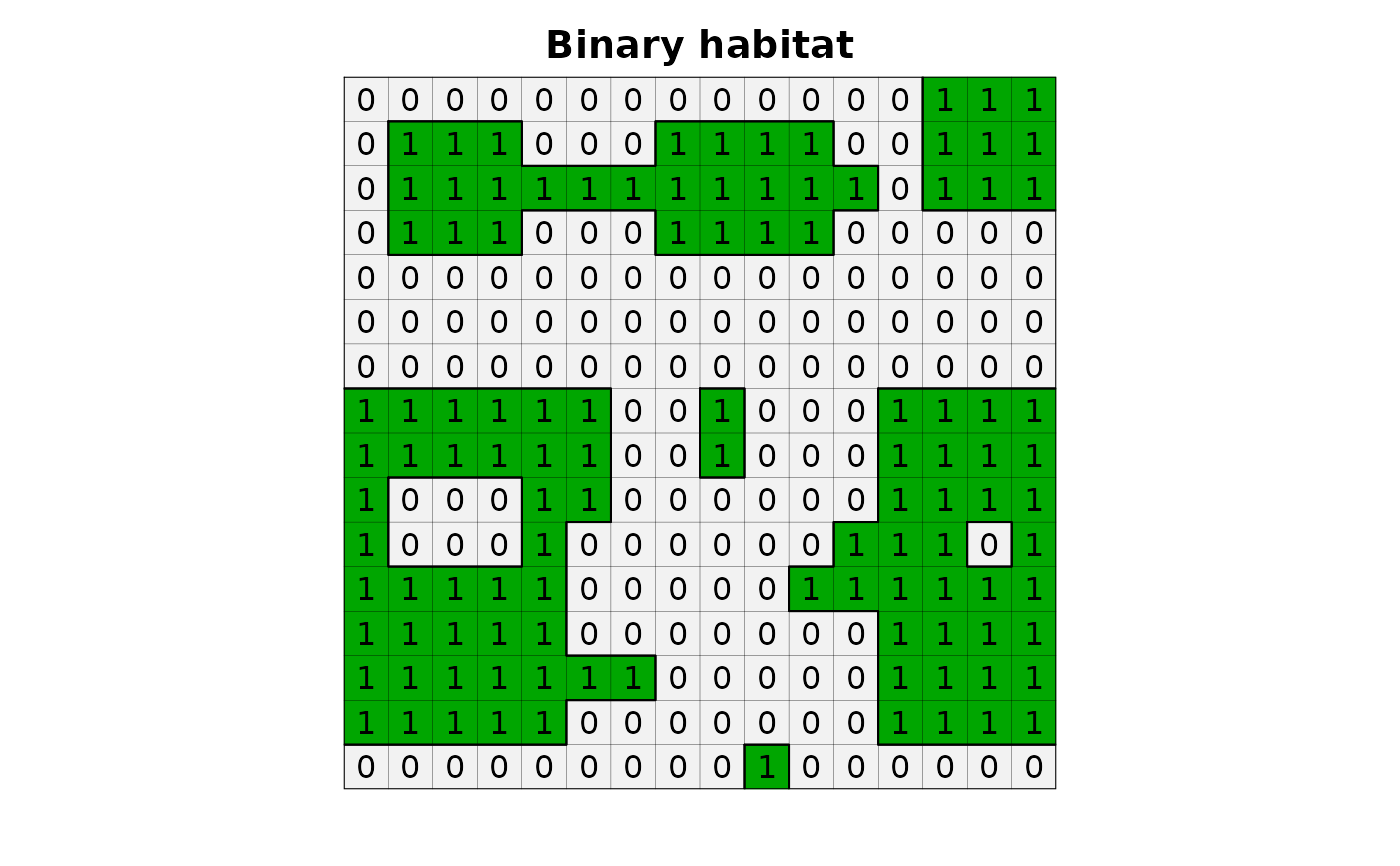
f <- system.file("raster/toy_landscape_habitat.tif", package = "lsmetrics")
r <- terra::rast(f)
# plot
plot(r, legend = FALSE, axes = FALSE, main = "Binary habitat")
plot(as.polygons(r, dissolve = FALSE), lwd = .1, add = TRUE)
plot(as.polygons(r), add = TRUE)
text(r)
 # find grass
path_grass <- system("grass --config path", inter = TRUE) # windows users need to find the grass gis path installation, e.g. "C:/Program Files/GRASS GIS 8.3"
# create grassdb
rgrass::initGRASS(gisBase = path_grass,
SG = r,
gisDbase = "grassdb",
location = "newLocation",
mapset = "PERMANENT",
override = TRUE)
#> gisdbase grassdb
#> location newLocation
#> mapset PERMANENT
#> rows 16
#> columns 16
#> north 7525600
#> south 7524000
#> west 234000
#> east 235600
#> nsres 100
#> ewres 100
#> projection:
#> PROJCRS["WGS 84 / UTM zone 23S",
#> BASEGEOGCRS["WGS 84",
#> ENSEMBLE["World Geodetic System 1984 ensemble",
#> MEMBER["World Geodetic System 1984 (Transit)"],
#> MEMBER["World Geodetic System 1984 (G730)"],
#> MEMBER["World Geodetic System 1984 (G873)"],
#> MEMBER["World Geodetic System 1984 (G1150)"],
#> MEMBER["World Geodetic System 1984 (G1674)"],
#> MEMBER["World Geodetic System 1984 (G1762)"],
#> MEMBER["World Geodetic System 1984 (G2139)"],
#> ELLIPSOID["WGS 84",6378137,298.257223563,
#> LENGTHUNIT["metre",1]],
#> ENSEMBLEACCURACY[2.0]],
#> PRIMEM["Greenwich",0,
#> ANGLEUNIT["degree",0.0174532925199433]],
#> ID["EPSG",4326]],
#> CONVERSION["UTM zone 23S",
#> METHOD["Transverse Mercator",
#> ID["EPSG",9807]],
#> PARAMETER["Latitude of natural origin",0,
#> ANGLEUNIT["degree",0.0174532925199433],
#> ID["EPSG",8801]],
#> PARAMETER["Longitude of natural origin",-45,
#> ANGLEUNIT["degree",0.0174532925199433],
#> ID["EPSG",8802]],
#> PARAMETER["Scale factor at natural origin",0.9996,
#> SCALEUNIT["unity",1],
#> ID["EPSG",8805]],
#> PARAMETER["False easting",500000,
#> LENGTHUNIT["metre",1],
#> ID["EPSG",8806]],
#> PARAMETER["False northing",10000000,
#> LENGTHUNIT["metre",1],
#> ID["EPSG",8807]]],
#> CS[Cartesian,2],
#> AXIS["(E)",east,
#> ORDER[1],
#> LENGTHUNIT["metre",1]],
#> AXIS["(N)",north,
#> ORDER[2],
#> LENGTHUNIT["metre",1]],
#> USAGE[
#> SCOPE["Navigation and medium accuracy spatial referencing."],
#> AREA["Between 48°W and 42°W, southern hemisphere between 80°S and equator, onshore and offshore. Brazil."],
#> BBOX[-80,-48,0,-42]],
#> ID["EPSG",32723]]
# import raster from r to grass
rgrass::write_RAST(x = r, flags = c("o", "overwrite", "quiet"), vname = "r")
#> SpatRaster read into GRASS using r.in.gdal from file
# functional connectivity
lsmetrics::lsm_functional_connectivity(input = "r", gap_crossing = 100, id = TRUE, dilation = TRUE)
#> Dilation pixels
#> Converting zero as null
#> Identifying the fragmentes for gap crossing
#> Multipling id by original habitat
#> Counting the number of fragmentes
#> Calculating the functional connected area
#> Converting zero as null
#> Identifying the fragmentes
#> Counting the cell number of fragmentes
#> First pass
#> 0% 6% 12% 18% 25% 31% 37% 43% 50% 56% 62% 68% 75% 81% 87% 93% 100%
#> Writing output map
#> 0% 6% 12% 18% 25% 31% 37% 43% 50% 56% 62% 68% 75% 81% 87% 93% 100%
#> Calculating the area of fragmentes
#> Removing extra rasters
# files
# rgrass::execGRASS(cmd = "g.list", type = "raster")
# import do r
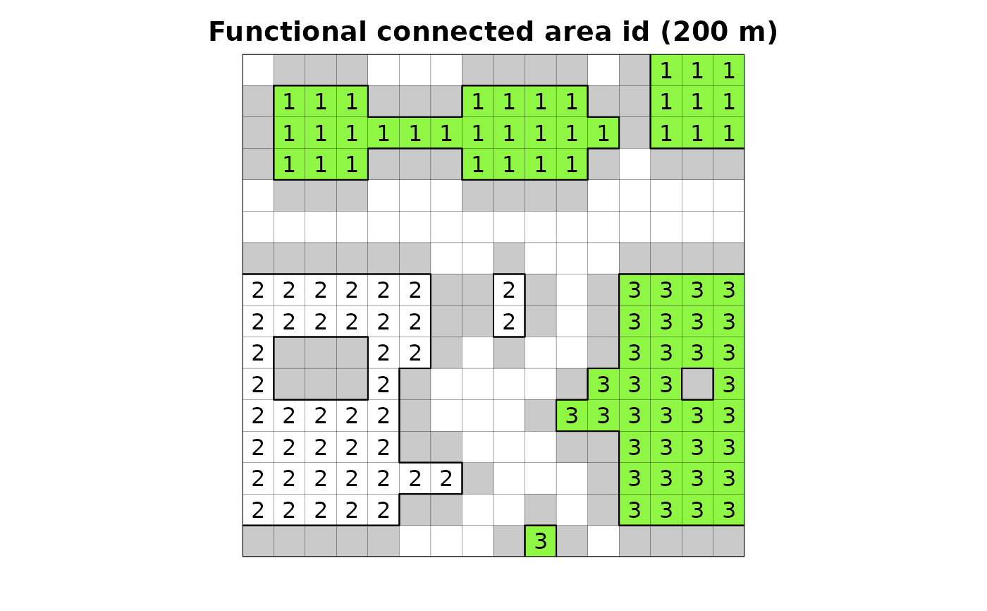
r_functional_connected_area200_id <- rgrass::read_RAST("r_functional_connected_area200_id", flags = "quiet", return_format = "terra")
r_functional_connectivity_dilation200_null <- rgrass::read_RAST("r_functional_connectivity_dilation200_null", flags = "quiet", return_format = "terra")
plot(r_functional_connectivity_dilation200_null, legend = FALSE, axes = FALSE,
main = "Functional connected area id (200 m)")
plot(r_functional_connected_area200_id, legend = FALSE, axes = FALSE, add = TRUE)
plot(as.polygons(r, dissolve = FALSE), lwd = .1, add = TRUE)
plot(as.polygons(r), add = TRUE)
text(r_functional_connected_area200_id)
# find grass
path_grass <- system("grass --config path", inter = TRUE) # windows users need to find the grass gis path installation, e.g. "C:/Program Files/GRASS GIS 8.3"
# create grassdb
rgrass::initGRASS(gisBase = path_grass,
SG = r,
gisDbase = "grassdb",
location = "newLocation",
mapset = "PERMANENT",
override = TRUE)
#> gisdbase grassdb
#> location newLocation
#> mapset PERMANENT
#> rows 16
#> columns 16
#> north 7525600
#> south 7524000
#> west 234000
#> east 235600
#> nsres 100
#> ewres 100
#> projection:
#> PROJCRS["WGS 84 / UTM zone 23S",
#> BASEGEOGCRS["WGS 84",
#> ENSEMBLE["World Geodetic System 1984 ensemble",
#> MEMBER["World Geodetic System 1984 (Transit)"],
#> MEMBER["World Geodetic System 1984 (G730)"],
#> MEMBER["World Geodetic System 1984 (G873)"],
#> MEMBER["World Geodetic System 1984 (G1150)"],
#> MEMBER["World Geodetic System 1984 (G1674)"],
#> MEMBER["World Geodetic System 1984 (G1762)"],
#> MEMBER["World Geodetic System 1984 (G2139)"],
#> ELLIPSOID["WGS 84",6378137,298.257223563,
#> LENGTHUNIT["metre",1]],
#> ENSEMBLEACCURACY[2.0]],
#> PRIMEM["Greenwich",0,
#> ANGLEUNIT["degree",0.0174532925199433]],
#> ID["EPSG",4326]],
#> CONVERSION["UTM zone 23S",
#> METHOD["Transverse Mercator",
#> ID["EPSG",9807]],
#> PARAMETER["Latitude of natural origin",0,
#> ANGLEUNIT["degree",0.0174532925199433],
#> ID["EPSG",8801]],
#> PARAMETER["Longitude of natural origin",-45,
#> ANGLEUNIT["degree",0.0174532925199433],
#> ID["EPSG",8802]],
#> PARAMETER["Scale factor at natural origin",0.9996,
#> SCALEUNIT["unity",1],
#> ID["EPSG",8805]],
#> PARAMETER["False easting",500000,
#> LENGTHUNIT["metre",1],
#> ID["EPSG",8806]],
#> PARAMETER["False northing",10000000,
#> LENGTHUNIT["metre",1],
#> ID["EPSG",8807]]],
#> CS[Cartesian,2],
#> AXIS["(E)",east,
#> ORDER[1],
#> LENGTHUNIT["metre",1]],
#> AXIS["(N)",north,
#> ORDER[2],
#> LENGTHUNIT["metre",1]],
#> USAGE[
#> SCOPE["Navigation and medium accuracy spatial referencing."],
#> AREA["Between 48°W and 42°W, southern hemisphere between 80°S and equator, onshore and offshore. Brazil."],
#> BBOX[-80,-48,0,-42]],
#> ID["EPSG",32723]]
# import raster from r to grass
rgrass::write_RAST(x = r, flags = c("o", "overwrite", "quiet"), vname = "r")
#> SpatRaster read into GRASS using r.in.gdal from file
# functional connectivity
lsmetrics::lsm_functional_connectivity(input = "r", gap_crossing = 100, id = TRUE, dilation = TRUE)
#> Dilation pixels
#> Converting zero as null
#> Identifying the fragmentes for gap crossing
#> Multipling id by original habitat
#> Counting the number of fragmentes
#> Calculating the functional connected area
#> Converting zero as null
#> Identifying the fragmentes
#> Counting the cell number of fragmentes
#> First pass
#> 0% 6% 12% 18% 25% 31% 37% 43% 50% 56% 62% 68% 75% 81% 87% 93% 100%
#> Writing output map
#> 0% 6% 12% 18% 25% 31% 37% 43% 50% 56% 62% 68% 75% 81% 87% 93% 100%
#> Calculating the area of fragmentes
#> Removing extra rasters
# files
# rgrass::execGRASS(cmd = "g.list", type = "raster")
# import do r
r_functional_connected_area200_id <- rgrass::read_RAST("r_functional_connected_area200_id", flags = "quiet", return_format = "terra")
r_functional_connectivity_dilation200_null <- rgrass::read_RAST("r_functional_connectivity_dilation200_null", flags = "quiet", return_format = "terra")
plot(r_functional_connectivity_dilation200_null, legend = FALSE, axes = FALSE,
main = "Functional connected area id (200 m)")
plot(r_functional_connected_area200_id, legend = FALSE, axes = FALSE, add = TRUE)
plot(as.polygons(r, dissolve = FALSE), lwd = .1, add = TRUE)
plot(as.polygons(r), add = TRUE)
text(r_functional_connected_area200_id)
 # import to r
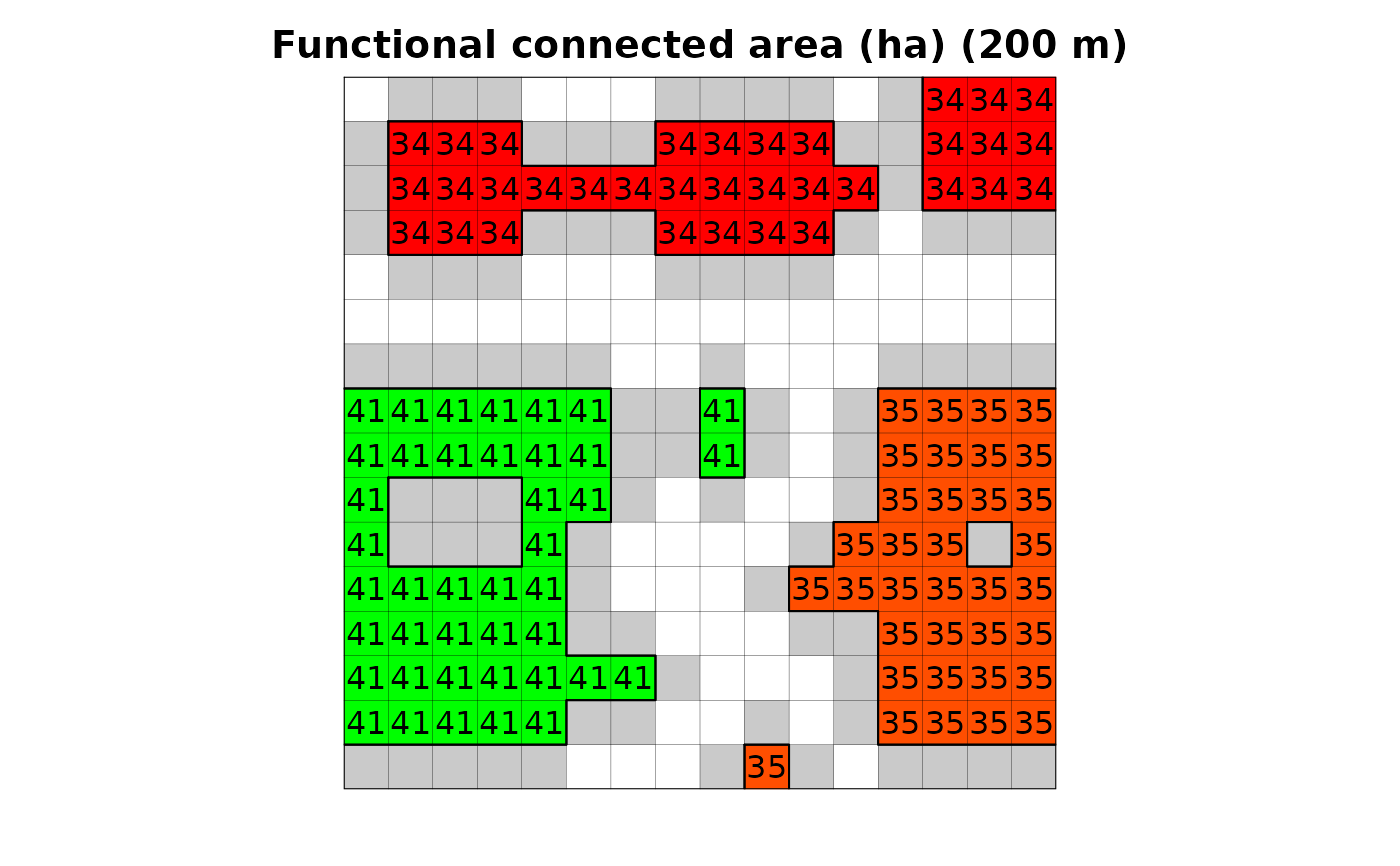
r_functional_connected_area200 <- rgrass::read_RAST("r_functional_connected_area200", flags = "quiet", return_format = "terra")
plot(r_functional_connectivity_dilation200_null, legend = FALSE, axes = FALSE,
main = "Functional connected area (ha) (200 m)")
plot(r_functional_connected_area200, legend = FALSE, axes = FALSE, add = TRUE)
plot(as.polygons(r, dissolve = FALSE), lwd = .1, add = TRUE)
plot(as.polygons(r), add = TRUE)
text(r_functional_connected_area200)
# import to r
r_functional_connected_area200 <- rgrass::read_RAST("r_functional_connected_area200", flags = "quiet", return_format = "terra")
plot(r_functional_connectivity_dilation200_null, legend = FALSE, axes = FALSE,
main = "Functional connected area (ha) (200 m)")
plot(r_functional_connected_area200, legend = FALSE, axes = FALSE, add = TRUE)
plot(as.polygons(r, dissolve = FALSE), lwd = .1, add = TRUE)
plot(as.polygons(r), add = TRUE)
text(r_functional_connected_area200)
 # import to r
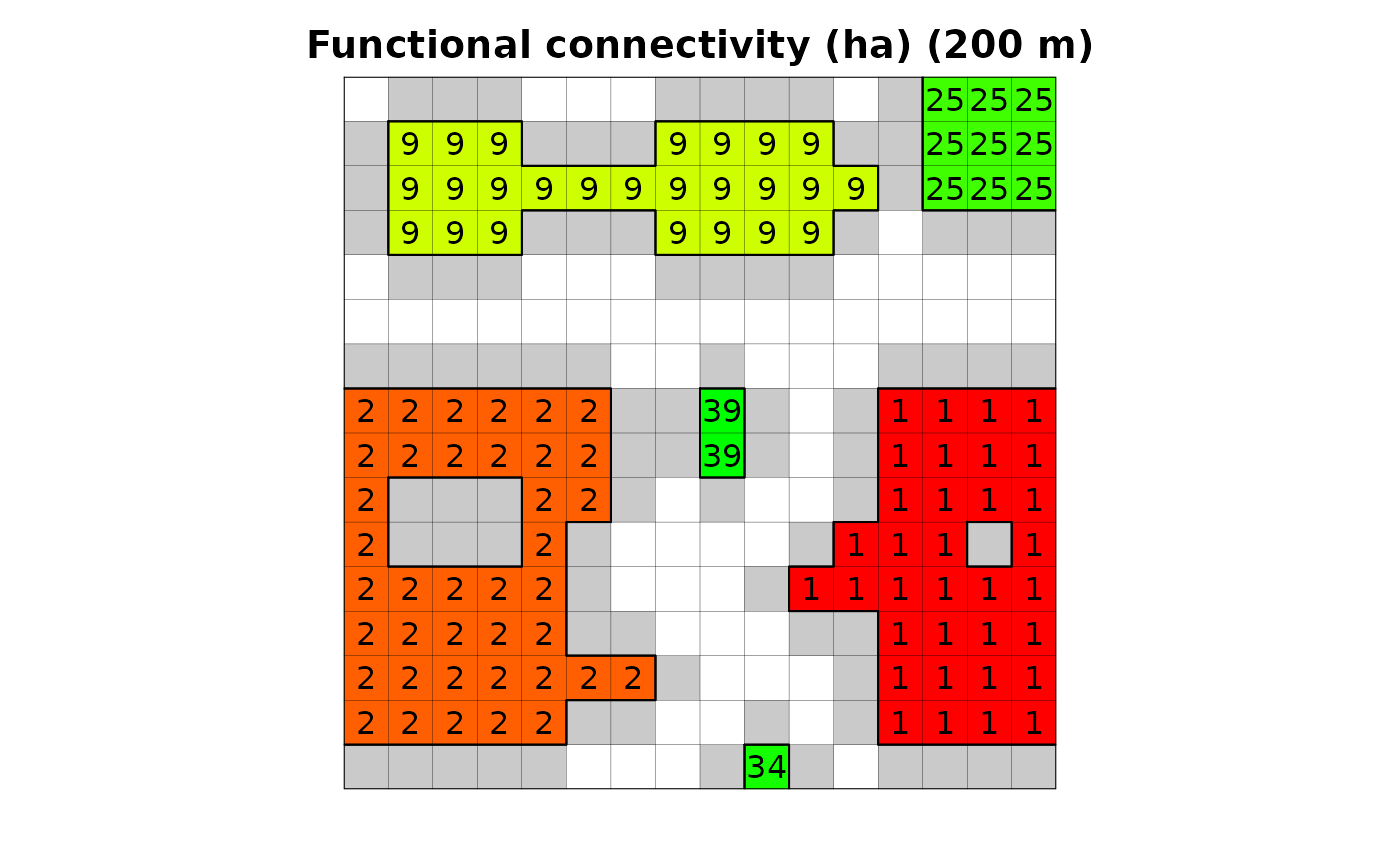
r_functional_connectivity200 <- rgrass::read_RAST("r_functional_connectivity200", flags = "quiet", return_format = "terra")
plot(r_functional_connectivity_dilation200_null, legend = FALSE, axes = FALSE,
main = "Functional connectivity (ha) (200 m)")
plot(r_functional_connectivity200, legend = FALSE, axes = FALSE, add = TRUE)
plot(as.polygons(r, dissolve = FALSE), lwd = .1, add = TRUE)
plot(as.polygons(r), add = TRUE)
text(r_functional_connectivity200)
# import to r
r_functional_connectivity200 <- rgrass::read_RAST("r_functional_connectivity200", flags = "quiet", return_format = "terra")
plot(r_functional_connectivity_dilation200_null, legend = FALSE, axes = FALSE,
main = "Functional connectivity (ha) (200 m)")
plot(r_functional_connectivity200, legend = FALSE, axes = FALSE, add = TRUE)
plot(as.polygons(r, dissolve = FALSE), lwd = .1, add = TRUE)
plot(as.polygons(r), add = TRUE)
text(r_functional_connectivity200)
 # delete grassdb
unlink("grassdb", recursive = TRUE)
# delete grassdb
unlink("grassdb", recursive = TRUE)