Calculate area.
Usage
lsm_aux_area(
  input_null,
  input_id,
  area_round_digit = 0,
  area_unit = "ha",
  map_ncell = FALSE,
  table_export = FALSE
)
Arguments
- input_null
[character=""]Habitat map (binary classification: e.g., 1/0 or 1/NA) in GRASS.- input_id
[character=""]Habitat map (binary classification: e.g., 1/0 or 1/NA) in GRASS.- area_round_digit
[integer]Decimal digits for area rounding.- area_unit
[character=""]Area unit:"ha","m2", or"km2".- map_ncell
[logical]Calculate number of cells.- table_export
[logical]Calculate number of cells.
Examples
library(lsmetrics)
library(terra)
# read habitat data
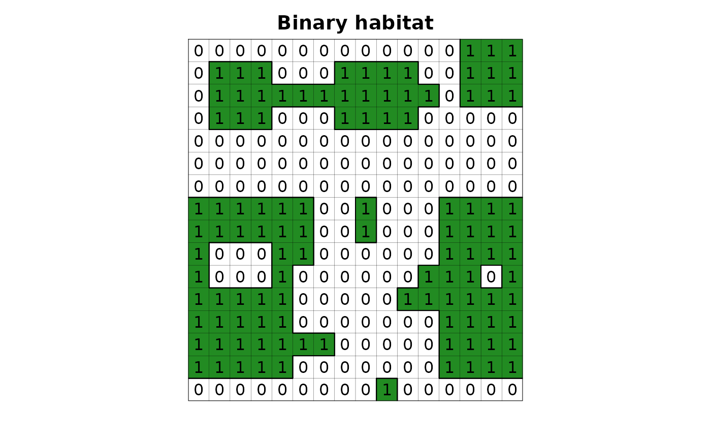
r <- lsmetrics::lsm_toy_landscape(proj_type = "meters")
# plot
plot(r, col = c("white", "forestgreen"), legend = FALSE, axes = FALSE, main = "Binary habitat")
plot(as.polygons(r, dissolve = FALSE), lwd = .1, add = TRUE)
plot(as.polygons(r), add = TRUE)
text(r)
 # find grass
path_grass <- system("grass --config path", inter = TRUE) # windows users need to find the grass gis path installation, e.g. "C:/Program Files/GRASS GIS 8.3"
# create grassdb
rgrass::initGRASS(gisBase = path_grass,
SG = r,
gisDbase = "grassdb",
location = "newLocation",
mapset = "PERMANENT",
override = TRUE)
#> gisdbase grassdb
#> location newLocation
#> mapset PERMANENT
#> rows 16
#> columns 16
#> north 7525600
#> south 7524000
#> west 234000
#> east 235600
#> nsres 100
#> ewres 100
#> projection:
#> PROJCRS["WGS 84 / UTM zone 23S",
#> BASEGEOGCRS["WGS 84",
#> ENSEMBLE["World Geodetic System 1984 ensemble",
#> MEMBER["World Geodetic System 1984 (Transit)"],
#> MEMBER["World Geodetic System 1984 (G730)"],
#> MEMBER["World Geodetic System 1984 (G873)"],
#> MEMBER["World Geodetic System 1984 (G1150)"],
#> MEMBER["World Geodetic System 1984 (G1674)"],
#> MEMBER["World Geodetic System 1984 (G1762)"],
#> MEMBER["World Geodetic System 1984 (G2139)"],
#> ELLIPSOID["WGS 84",6378137,298.257223563,
#> LENGTHUNIT["metre",1]],
#> ENSEMBLEACCURACY[2.0]],
#> PRIMEM["Greenwich",0,
#> ANGLEUNIT["degree",0.0174532925199433]],
#> ID["EPSG",4326]],
#> CONVERSION["UTM zone 23S",
#> METHOD["Transverse Mercator",
#> ID["EPSG",9807]],
#> PARAMETER["Latitude of natural origin",0,
#> ANGLEUNIT["degree",0.0174532925199433],
#> ID["EPSG",8801]],
#> PARAMETER["Longitude of natural origin",-45,
#> ANGLEUNIT["degree",0.0174532925199433],
#> ID["EPSG",8802]],
#> PARAMETER["Scale factor at natural origin",0.9996,
#> SCALEUNIT["unity",1],
#> ID["EPSG",8805]],
#> PARAMETER["False easting",500000,
#> LENGTHUNIT["metre",1],
#> ID["EPSG",8806]],
#> PARAMETER["False northing",10000000,
#> LENGTHUNIT["metre",1],
#> ID["EPSG",8807]]],
#> CS[Cartesian,2],
#> AXIS["(E)",east,
#> ORDER[1],
#> LENGTHUNIT["metre",1]],
#> AXIS["(N)",north,
#> ORDER[2],
#> LENGTHUNIT["metre",1]],
#> USAGE[
#> SCOPE["Navigation and medium accuracy spatial referencing."],
#> AREA["Between 48°W and 42°W, southern hemisphere between 80°S and equator, onshore and offshore. Brazil."],
#> BBOX[-80,-48,0,-42]],
#> ID["EPSG",32723]]
# import raster from r to grass
rgrass::write_RAST(x = r, flags = c("o", "overwrite", "quiet"), vname = "r", verbose = FALSE)
# null
rgrass::execGRASS(cmd = "r.mapcalc", flags = "overwrite", expression = "r_null = if(r == 1, 1, null())")
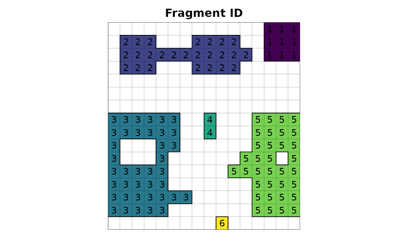
# clump
rgrass::execGRASS(cmd = "r.clump", flags = "overwrite", input = "r_null", output = "r_id")
#> Pass 1 of 2...
#> 0% 6% 12% 18% 25% 31% 37% 43% 50% 56% 62% 68% 75% 81% 87% 93% 100%
#> Generating renumbering scheme...
#> 0% 11% 22% 33% 44% 55% 66% 77% 88% 100%
#> Pass 2 of 2...
#> 0% 6% 12% 18% 25% 31% 37% 43% 50% 56% 62% 68% 75% 81% 87% 93% 100%
#> r.clump complete. 6 clumps.
# area
lsmetrics::lsm_aux_area(input_null = "r_null",
input_id = "r_id",
area_round_digit = 0,
area_unit = "ha",
map_ncell = TRUE,
table_export = TRUE)
#> Cell counting
#> First pass
#> 0% 6% 12% 18% 25% 31% 37% 43% 50% 56% 62% 68% 75% 81% 87% 93% 100%
#> Writing output map
#> 0% 6% 12% 18% 25% 31% 37% 43% 50% 56% 62% 68% 75% 81% 87% 93% 100%
#> Mask creating
#> Area calculating
#> First pass
#> 0% 6% 12% 18% 25% 31% 37% 43% 50% 56% 62% 68% 75% 81% 87% 93% 100%
#> Writing output map
#> 0% 6% 12% 18% 25% 31% 37% 43% 50% 56% 62% 68% 75% 81% 87% 93% 100%
#> Color assigning
#> Table exporting
# files
rgrass::execGRASS(cmd = "g.list", type = "raster")
#> r
#> r_id
#> r_null
#> r_null_area
#> r_null_ncell
# plot
r_id <- terra::rast(rgrass::read_RAST("r_id", flags = "quiet", return_format = "SGDF"))
#> Creating BIL support files...
#> Exporting raster as integer values (bytes=4)
#> 0% 6% 12% 18% 25% 31% 37% 43% 50% 56% 62% 68% 75% 81% 87% 93% 100%
plot(r_id, legend = FALSE, axes = FALSE, main = "Fragment ID")
plot(as.polygons(r, dissolve = FALSE), lwd = .1, add = TRUE)
plot(as.polygons(r), add = TRUE)
text(r_id)
# find grass
path_grass <- system("grass --config path", inter = TRUE) # windows users need to find the grass gis path installation, e.g. "C:/Program Files/GRASS GIS 8.3"
# create grassdb
rgrass::initGRASS(gisBase = path_grass,
SG = r,
gisDbase = "grassdb",
location = "newLocation",
mapset = "PERMANENT",
override = TRUE)
#> gisdbase grassdb
#> location newLocation
#> mapset PERMANENT
#> rows 16
#> columns 16
#> north 7525600
#> south 7524000
#> west 234000
#> east 235600
#> nsres 100
#> ewres 100
#> projection:
#> PROJCRS["WGS 84 / UTM zone 23S",
#> BASEGEOGCRS["WGS 84",
#> ENSEMBLE["World Geodetic System 1984 ensemble",
#> MEMBER["World Geodetic System 1984 (Transit)"],
#> MEMBER["World Geodetic System 1984 (G730)"],
#> MEMBER["World Geodetic System 1984 (G873)"],
#> MEMBER["World Geodetic System 1984 (G1150)"],
#> MEMBER["World Geodetic System 1984 (G1674)"],
#> MEMBER["World Geodetic System 1984 (G1762)"],
#> MEMBER["World Geodetic System 1984 (G2139)"],
#> ELLIPSOID["WGS 84",6378137,298.257223563,
#> LENGTHUNIT["metre",1]],
#> ENSEMBLEACCURACY[2.0]],
#> PRIMEM["Greenwich",0,
#> ANGLEUNIT["degree",0.0174532925199433]],
#> ID["EPSG",4326]],
#> CONVERSION["UTM zone 23S",
#> METHOD["Transverse Mercator",
#> ID["EPSG",9807]],
#> PARAMETER["Latitude of natural origin",0,
#> ANGLEUNIT["degree",0.0174532925199433],
#> ID["EPSG",8801]],
#> PARAMETER["Longitude of natural origin",-45,
#> ANGLEUNIT["degree",0.0174532925199433],
#> ID["EPSG",8802]],
#> PARAMETER["Scale factor at natural origin",0.9996,
#> SCALEUNIT["unity",1],
#> ID["EPSG",8805]],
#> PARAMETER["False easting",500000,
#> LENGTHUNIT["metre",1],
#> ID["EPSG",8806]],
#> PARAMETER["False northing",10000000,
#> LENGTHUNIT["metre",1],
#> ID["EPSG",8807]]],
#> CS[Cartesian,2],
#> AXIS["(E)",east,
#> ORDER[1],
#> LENGTHUNIT["metre",1]],
#> AXIS["(N)",north,
#> ORDER[2],
#> LENGTHUNIT["metre",1]],
#> USAGE[
#> SCOPE["Navigation and medium accuracy spatial referencing."],
#> AREA["Between 48°W and 42°W, southern hemisphere between 80°S and equator, onshore and offshore. Brazil."],
#> BBOX[-80,-48,0,-42]],
#> ID["EPSG",32723]]
# import raster from r to grass
rgrass::write_RAST(x = r, flags = c("o", "overwrite", "quiet"), vname = "r", verbose = FALSE)
# null
rgrass::execGRASS(cmd = "r.mapcalc", flags = "overwrite", expression = "r_null = if(r == 1, 1, null())")
# clump
rgrass::execGRASS(cmd = "r.clump", flags = "overwrite", input = "r_null", output = "r_id")
#> Pass 1 of 2...
#> 0% 6% 12% 18% 25% 31% 37% 43% 50% 56% 62% 68% 75% 81% 87% 93% 100%
#> Generating renumbering scheme...
#> 0% 11% 22% 33% 44% 55% 66% 77% 88% 100%
#> Pass 2 of 2...
#> 0% 6% 12% 18% 25% 31% 37% 43% 50% 56% 62% 68% 75% 81% 87% 93% 100%
#> r.clump complete. 6 clumps.
# area
lsmetrics::lsm_aux_area(input_null = "r_null",
input_id = "r_id",
area_round_digit = 0,
area_unit = "ha",
map_ncell = TRUE,
table_export = TRUE)
#> Cell counting
#> First pass
#> 0% 6% 12% 18% 25% 31% 37% 43% 50% 56% 62% 68% 75% 81% 87% 93% 100%
#> Writing output map
#> 0% 6% 12% 18% 25% 31% 37% 43% 50% 56% 62% 68% 75% 81% 87% 93% 100%
#> Mask creating
#> Area calculating
#> First pass
#> 0% 6% 12% 18% 25% 31% 37% 43% 50% 56% 62% 68% 75% 81% 87% 93% 100%
#> Writing output map
#> 0% 6% 12% 18% 25% 31% 37% 43% 50% 56% 62% 68% 75% 81% 87% 93% 100%
#> Color assigning
#> Table exporting
# files
rgrass::execGRASS(cmd = "g.list", type = "raster")
#> r
#> r_id
#> r_null
#> r_null_area
#> r_null_ncell
# plot
r_id <- terra::rast(rgrass::read_RAST("r_id", flags = "quiet", return_format = "SGDF"))
#> Creating BIL support files...
#> Exporting raster as integer values (bytes=4)
#> 0% 6% 12% 18% 25% 31% 37% 43% 50% 56% 62% 68% 75% 81% 87% 93% 100%
plot(r_id, legend = FALSE, axes = FALSE, main = "Fragment ID")
plot(as.polygons(r, dissolve = FALSE), lwd = .1, add = TRUE)
plot(as.polygons(r), add = TRUE)
text(r_id)
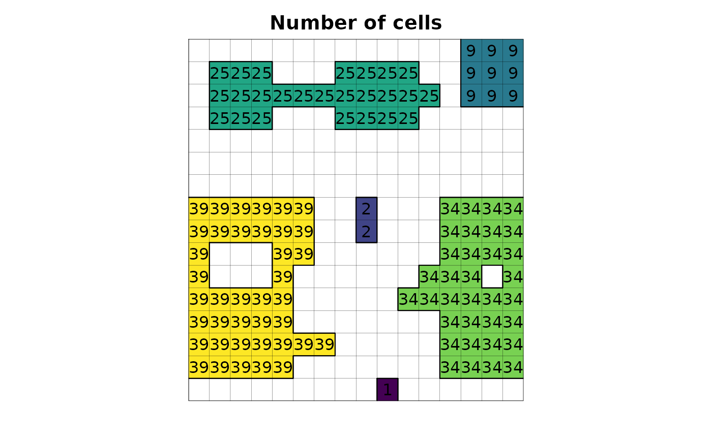
 r_ncell <- terra::rast(rgrass::read_RAST("r_null_ncell", flags = "quiet", return_format = "SGDF"))
#> Creating BIL support files...
#> Exporting raster as floating values (bytes=4)
#> 0% 6% 12% 18% 25% 31% 37% 43% 50% 56% 62% 68% 75% 81% 87% 93% 100%
plot(r_ncell, legend = FALSE, axes = FALSE, main = "Number of cells")
plot(as.polygons(r, dissolve = FALSE), lwd = .1, add = TRUE)
plot(as.polygons(r), add = TRUE)
text(r_ncell)
r_ncell <- terra::rast(rgrass::read_RAST("r_null_ncell", flags = "quiet", return_format = "SGDF"))
#> Creating BIL support files...
#> Exporting raster as floating values (bytes=4)
#> 0% 6% 12% 18% 25% 31% 37% 43% 50% 56% 62% 68% 75% 81% 87% 93% 100%
plot(r_ncell, legend = FALSE, axes = FALSE, main = "Number of cells")
plot(as.polygons(r, dissolve = FALSE), lwd = .1, add = TRUE)
plot(as.polygons(r), add = TRUE)
text(r_ncell)
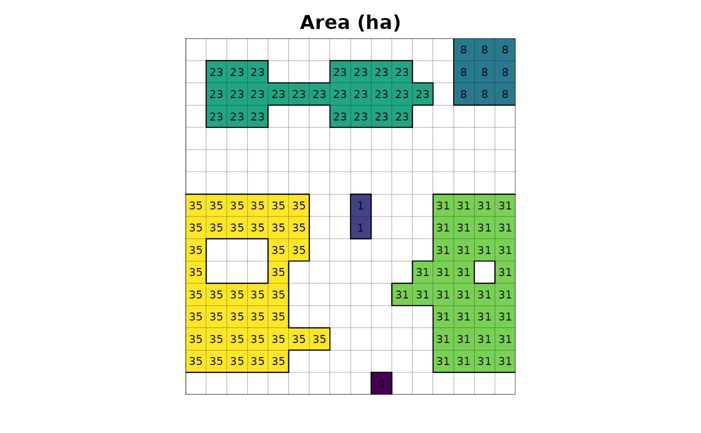
 r_area <- terra::rast(rgrass::read_RAST("r_null_area", flags = "quiet", return_format = "SGDF"))
#> Creating BIL support files...
#> Exporting raster as integer values (bytes=4)
#> 0% 6% 12% 18% 25% 31% 37% 43% 50% 56% 62% 68% 75% 81% 87% 93% 100%
plot(r_area, legend = FALSE, axes = FALSE, main = "Area (ha)")
plot(as.polygons(r, dissolve = FALSE), lwd = .1, add = TRUE)
plot(as.polygons(r), add = TRUE)
text(r_area, cex = .7, digits = 3)
r_area <- terra::rast(rgrass::read_RAST("r_null_area", flags = "quiet", return_format = "SGDF"))
#> Creating BIL support files...
#> Exporting raster as integer values (bytes=4)
#> 0% 6% 12% 18% 25% 31% 37% 43% 50% 56% 62% 68% 75% 81% 87% 93% 100%
plot(r_area, legend = FALSE, axes = FALSE, main = "Area (ha)")
plot(as.polygons(r, dissolve = FALSE), lwd = .1, add = TRUE)
plot(as.polygons(r), add = TRUE)
text(r_area, cex = .7, digits = 3)
 # table
r_table_area <- vroom::vroom("r_null_table_area.csv", show_col_types = FALSE)
r_table_area
#> # A tibble: 6 × 3
#> id area ncell
#> <dbl> <dbl> <dbl>
#> 1 1 9 9
#> 2 2 25 25
#> 3 3 39 39
#> 4 4 2 2
#> 5 5 34 34
#> 6 6 1 1
# delete table and grassdb
unlink("r_table_area.csv")
unlink("grassdb", recursive = TRUE)
# table
r_table_area <- vroom::vroom("r_null_table_area.csv", show_col_types = FALSE)
r_table_area
#> # A tibble: 6 × 3
#> id area ncell
#> <dbl> <dbl> <dbl>
#> 1 1 9 9
#> 2 2 25 25
#> 3 3 39 39
#> 4 4 2 2
#> 5 5 34 34
#> 6 6 1 1
# delete table and grassdb
unlink("r_table_area.csv")
unlink("grassdb", recursive = TRUE)